sys-design-interview.github.io
Metrics monitoring system
Table of contents
- Question
- Clarifying questions
- Scale and estimates
- Metric definition
- Metrics ingestion: push vs. pull
- High level design
- Components and responsibilities
- Deep dive: Persistent store
- Deep dive: Compactions, downsampling
- Potential improvements
- References
- Note to readers
Question
Design a metrics monitoring system.
Clarifying questions
Candidate: (understanding the use-case) Is this a system which is used to
monitor, export and visualize some key metrics (eg, RAM, CPU etc) in their servers.
Interviewer: Yes. Imagine a medium-sized company (for now) that runs multiple
services in a fleet of machines.
Candidate: Ok, I am familiar with such a system. I assume we should also allow
application-developers to compute and export custom metrics? (for eg, num-requests)?
Interviewer: Yes, that is also a key requirement.
Candidate: I have some more questions:
- how long should the metrics be persisted?
- is this system primarily for use internally within the company? Or should
we expect external services to be monitored as well? - what are the types of jobs being monitored? Are these continously running
jobs? Or should we design it primarily for monitoring batch jobs’ metrics? - is alerting also in scope of this design?
Interviewer:
- the metrics should be persisted for 2 years, as these could be used by devs
for debugging some trends. - yes, we can assume that the machines monitored will be internal to the company.
- batch jobs are lower priority for now. We can focus on continuously running
jobs. - alerting is lower priority for now. We can get to it if we have time.
Scale and estimates
Candidate: How many machines are in the fleet? How many metrics can we expect
to collect from each machine?
Interviewer: Let us assume that there are 10k machines in the fleet, and
we collect about ~1k metrics per machine.
Candidate: Assuming we collect metrics every second from each machine, that
gives us: 1k metrics per machine * 10k machines = 10M data points per second.
Also, we have a requirement that these data points should be persisted for 2 years.
Given that requirement, we need to be able to ingest metrics at the rate of 10M
per second. This system is write-heavy.
Just to clarify, the primary users of the data are developers in the company, right?
So, can we assume that there will be relatively lower number of reads, say 1k per
second?
Interviewer: Yes, you can assume 1k reads per second.
Metric definition
Candidate: At this point, it might be useful to get on the same page about
what we mean by a “metric”. Here’s what I am thinking:
- A metric will be of the format:
<machine_id>.<service_name>.<metric_name>{tag1=val1, tag2=val2, ...} - It is always associated with a timestamp
- It will always have a value (
int,float,stringetc.) - “Tags” are arbitrary key-value pairs that can be attached to the metric. This
could be application-specific and are primarily used by developers to slice
the metrics. For example, select only “premium” users’ queries, or look at
metrics of users from the USA. We should be able to support multiple such tags.
Example: 0.my_service.num_requests{country=us, user_class=premium} may have a
value of 12345 and may be associated with a timestamp 1234567890.
In the above metric, “0” is the machine-id. This is to differentiate different
machines that are running the same service.
Interviewer: Yes this is quite standard. Looks ok to me.
Metrics ingestion: push vs. pull
Candidate: Before getting to the high-level-design, I would like to discuss
the options we have to actually ingest the data into our system.
Push approach
In this approach, we provide APIs and client libraries, which the machines would
use to send the metrics over to our system.
Pros:
- works for both batch-jobs and continuously-running servers with the same API.
- for batch jobs, the application code can push the metrics once it is done (just
before exiting).
- for batch jobs, the application code can push the metrics once it is done (just
- better for systems which may be behind firewall. If so, “pull” approach might
be tricky, as we will have to make some changes in our “puller” to get past the
firewall.
Cons:
- ingestion rate might be difficult to control as some clients can push too many
metrics, too fast. - integration with clients might be more difficult, as the clients’ machines
would have to know where to push to.
Pull approach
In this approach, we let the client machines compute the metrics in memory and
expose them via an HTTP endpoint. For example, something like http://my-service/metrics
That way, we can maintain a set of “collectors” who scrape metrics for each service
from the /metrics endpoint.
Pros:
- Client integration is slightly easier, as they just have to expose the metrics
at a particular place. The monitoring system does the collection and storage. - We can throttle/control the ingestion rate, and hence have lesser risk of getting
overwhelmed.
Cons:
- Pull based approach won’t work well if the machines we want to monitor are behind
a firewall (not an issue for fleet inside the company’s network) - We need to do service discovery and maintain the mapping between our set of
“collectors” and the list of target-machines to be scraped. This adds complexity
(while simplifying client integration).
Decision: pull approach
Candidate: I’d like to take the pull-based approach, as it satisfies our initial
constraints (no batch jobs, machines inside company’s network), and has scope for
faster client integration.
Interviewer: Hmmm, ok.
High level design
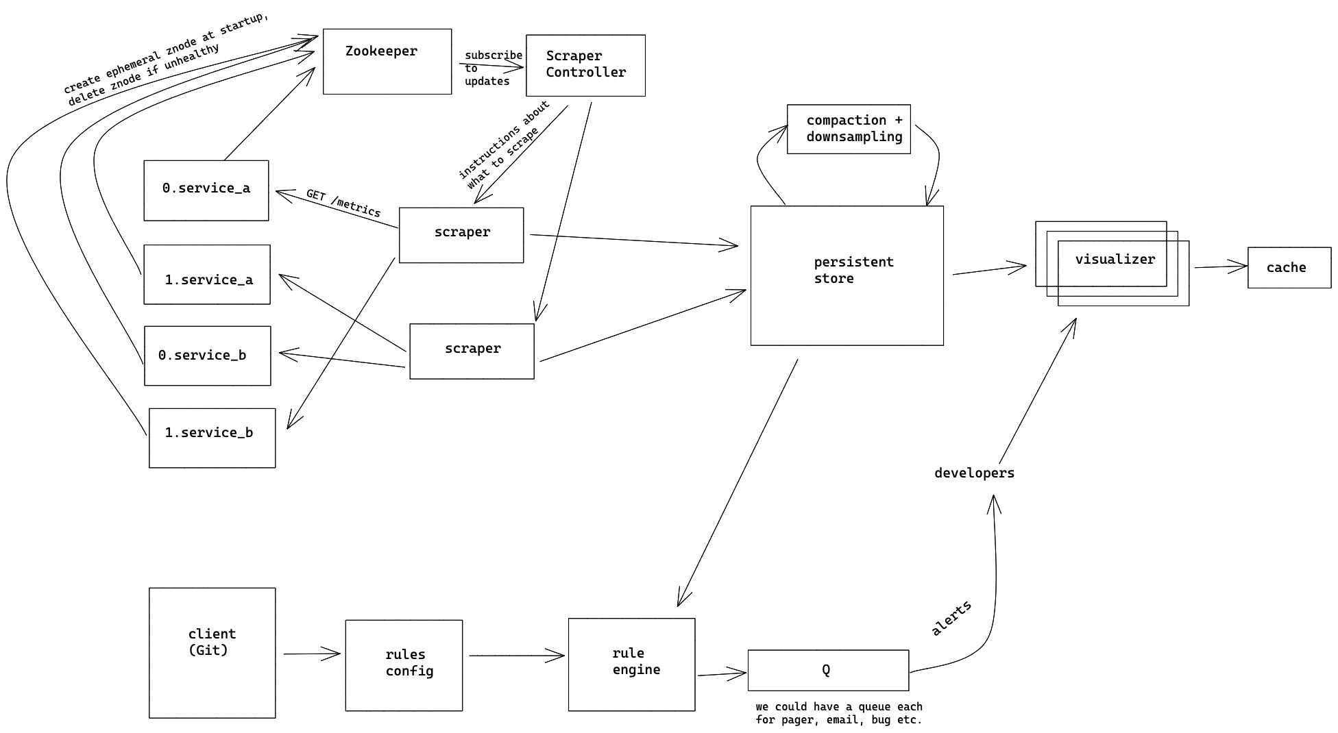
Components and responsibilities
Candidate: Here are the high-level components and their responsiblities:
External services
These are groups of machines which arerepresent external services. For this design
they are represented in the form of <machine_id>.<service_name>. These are
the machines which we want to monitor.
Note that these machines would export their computed metrics via a /metrics
HTTP endpoint, so that the metrics can be scraped.
Scraper
Since our ingestion mechanism is pull-based, we need a set of machines to scrape
the metrics from external services. It is unlikely that we can scrape all services
using just a single machine. So, we’d have a set of scrapers to do this job for us.
Now that we have 2 sets of machines (one for a set of services, and other for
scraping those machines), we need to have some kind of assignment between these.
Specifically, a single scraper instance pulls metrics from a list of “target” machines.
The list of target machines is sharded across multiple scrapers based on the
hash of machine’s IP address. The mapping from scraper to list-of-target-machines
can be maintained in Zookeeper.
The scraper’s main task is to keep collecting metrics from each target-machine
that is assigned to it at a certain interval (say, every second) and push them
to the persistent store.
Apart from that, it listens to instructions from the “ScrapperController” about
any new additions to target-machines, or redistribution of work in case of new
scrapers being added/deleted.
Scraper Controller
This component manages the mapping from Scraper instances to the list of target
machines to scrape for each instance. Some responsibilities of this component are:
- detect/re-assign set of target-machines
- detect additions/deletions of scraper instances and redistribute work among them.
The controller does this by using Zookeeper as its source of truth about the
list of target-machines and scraper instances and getting notified if any instance
gets added or removed from the fleet. The controller does not actually do any
scrapping, but sends directives to scrapers about what they should do.
For resilience, we can have multiple replicas of controllers, with a single
master-elected instance of the controller actually sending the directives and
updating Zookeeper about the mapping information.
Persistent store
This is the place where all metrics will be ingested, and stored persistently.
We will go into details about the store in our deep-dives.
Visualizer
This would be the server which processes the queries made by developers and returns
timeseries as a result for those queries. They could be stateless replicas
which talk to the persistent store to get the underlying timeseries data. To
prevent hitting the persistent store again and again, we could have an in-memory
LRU cache in each instance of the visualizer server.
Alerting system
The alerting system consists of:
- rules-config store which maintains a list of alerting rules submitted by the
developers. These could be in a specific language, specifying which metric to
monitor, what criteria should be met in order to trigger the alert, and the
severity of the alert (pager, email etc.) along with its destination. - rules engine, which constantly evaluates the rules at regular intervals, and
enqueues the alerts in the appropriate queue (based on severity) if needed. - worker component which dequeues items from the queue and delivers the alerts.
Since this is lower priority in our design, we may not fully flesh out this design.
Candidate: That is a high-level overview of the system. I’d like to
talk more about the persistent-store since we should design it in such a way
that it supports millions of writes per second.
Interviewer: Sounds good.
Deep dive: Persistent store
Candidate: Let us first start by discussing what type of store would fit our
use-case here. The characteristics of the incoming writes are as follows:
- very high rate of writes (millions per second)
- no complex relationships between data (we have a metric name, and the value)
- no mutations on the data.
- once a metric is recorded, we don’t need to change it later. It is almost
like an append-only log of timeseries data.
- once a metric is recorded, we don’t need to change it later. It is almost
- all queries will be time-based.
- this indicates that we need the retrieval to be good at range-scanning.
Given the above, a NoSQL, wide-column datastore like Bigtable/HBase seems like a
good choice to me. We should have the “key” of our persistent-store contain a
timestamp. That way, we can do efficient range-scans, which is exactly what we
need to render the visualizations of the metrics.
This is how we’d structure the persistent store:
Key: <machine_id>.<service_name>.<metric_name>.<timestamp_rounded_to_hour>.<tag1>=<val1>...<tagN>=<valN>
Column families: For now, we may need only 1 column family. Let us call it “data”.
Assuming that we collect metrics every second, each row can have 3600 columns, one
for each second. That way, a metric collected at time, say 10:00:35 PM would be written
as:
| Key | +0 | +1 | +2 | +3 | … | +35 | … | +3600 |
|---|---|---|---|---|---|---|---|---|
0.service_a.cpu.10pm |
- | - | - | - | - | 123 | - | - |
1.service_a.cpu.10pm |
- | - | - | - | - | 4 | - | - |
2.service_a.cpu.10pm |
- | - | - | - | - | 3 | - | - |
Note that:
- the “key” contains “10pm” (which would actually be a timestamp, rounded to the
nearest hour) - the column “+35” contains the actual recorded value for the
cpumetric.
Similarly, as new values come in, they will just be written to their respective
columns.
The main advantage of such a schema is that each row of the bigtable contains
one hour’s worth of information. So, for a lot of the queries, we would need to
read only a handful of rows, making the queries faster.
Interviewer: Interesting. Why is the “timestamp” component of the “key” at
the very end here? Wouldn’t it affect range-query performance?
Candidate: We should be wary of hot-spotting when deciding the key schema
for HBase/BigTable.
Note that, internally, BigTable/HBase store keys with similar prefix in the same
machine. So, writes/reads to such similar prefixes will also land in those machines.
This could lead to hot-spots.
If we have timestamp as the first component in the key, then all metrics of all
services will be written to the rows starting with timestamp. Hence, they will
land in a very small set of machines which own the data starting with that prefix,
leading to hot-spots. To avoid this, we want to spread the writes coming in from
all the machines’ metrics as randomly as possible inside BigTable/HBase. Having
metric_name and service_name will increase the chances of spreading out those
writes.
Also note, adding this to the key-prefix would not negatively affect our query
performance. This is because, we already know the exact prefixes to query. For
example, the developers would already provide the service_name and the metric_name
they are interested in (along with the time-range). So, our visualizer servers
can construct a BigTable/HBase query based on those inputs. Inside the BigTable,
those keys we are querying for are likely to be co-located in the same backend servers.
Interviewer: I see. What about the tags, though? They are at the very end of
the key. How would the queries for tags perform?
Candidate: Good point. Let’s say the developer is interested in querying
for num-requests originating permium-users in us, for example.
Developer’s input would be: my_service.num_requests{country=us, user_type=premium}
In this case, the visualizer server should append some regex based on the tags
like country.*us.*user_type.*premium at the end of the BigTable query. BigTable
has native support for filtering data using regexes (in the BigTable’s backend).
This is usually quicker than the clients retrieving the results and filtering
out the rows. That being said, yes, one downside of this approach is that querying
with multiple tags could be slow.
However, in practice, we do not expect developers to add a lot of tags in their
regular queries – so this might be ok.
If we have time, I can revisit this to see if we can make this faster for at least
some types of queries.
For now, I’d like to talk about some data optimizations that we can perform on
the persistent store.
Interviewer: Ok.
Deep dive: Compactions, downsampling
Saving disk space
When we store the metrics across 3600 columns, BigTable/HBase stores the key
for each entry along with the value. This leads to potential inefficiency, as the
same key is stored ~3600 times. In order to save space, we can take advantage of
the immutable property of the metrics data here. After the hour passes by, we know
we will not mutate that row’s data. So, we can just merge all the columns’ data
into one blob (maybe in json format) and write it into a separate column.
| Key | +0 | +1 | +2 | … | +35 | … | +3600 | blob |
|---|---|---|---|---|---|---|---|---|
0.service_a.cpu.10pm |
… | - | … | {0:1 1:4 2:7 ...} |
The numbers that have been struck-through above are “deleted” and added to the “blob”
column in the persistent store. Note that “deleting” data in a column will add a
tombstone, which will then be cleaned up later by BigTable’s compaction process
(different from what is being described here).
Downsampling
Note that we would be storing all data at the granularity of seconds when the
data is being ingested realtime. When querying over long time-ranges (say, a year),
the number of points returned to the front-end/client will be very large. Also,
it is very likely that the developers aren’t interested in knowing second-by-second
information about their query over such a large timerange. On top of that, the
client can also get overwhelmed by this data.
To solve this, we have to downsample. There are 2 options here:
- Downsample at client side (return all the second-by-second results to the client)
- Downsample at the server side. (run a batch job to reduce the number of points)
I’d prefer option 2 as it is more efficient (because we won’t send all the data
over the wire, and it will render quickly on the client, without requiring additional
processing).
For downsampling, we can run batch jobs which look at the last few hours of data
(say, 4 hours) and select only the “interesting points” and write them out in a
column. The selection of “interesting” points is probably a separate topic in itself,
but for the first version, I’d just do random sampling of points.
To perform both compactions and downsampling, we need to have a set of machines
which run in batch mode by reading data from persistent-store and writing out
processed data back to it.
The querying logic should also be aware that the downsampled data exists. So,
if the timerange of the incoming query is spanning more than 4 hours, we should
direct the query for the anything before 4 hours to read the downsampled column.
Interviewer: That sounds like a good idea. We’re out of time. Thanks!
Potential improvements
- Instead of ingesting all the points immediately to persistent store, have a
tiered storage approach:- data for the last ~4 hours are stored in memory (with write-ahead-log)
- after that, it is moved to bigtable (using the data in write-ahead-log)
- data more than ~6-12 months can be moved to even cheaper storage (if available)
- querying should be aware of these tiers and send+collect the results accordingly.
- Flesh out the alerting system design.
References
Note to readers
If you see any issues with the existing approach, or would like to suggest
improvements, please send an email to contact@sys-design-interview.com, or comment
below. Always ready to accept feedback and improve!